finite element preliminaries

This blog post presents some of the finite element theory used in the section properties program in a simplified and easy to understand manner. It is worth noting that the notions used in the section properties program are the same that are applied in commercial finite element solvers. For a more in-depth overview of the section properties program, check out the paper I wrote here.

Breaking it down

The finite element method simplifies a complex problem by breaking it down into a large number of smaller, workable problems. For this reason, the finite element method lends itself nicely to the development of a program that can handle any imaginable cross-section.

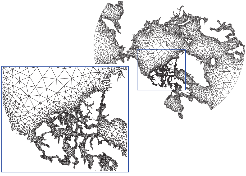
In the case of a structural cross-section, any arbitrary enclosed shape can easily (with the aid of a meshing algorithm) be broken down into a collection of smaller, simple shapes. The shape that is the easiest to mesh and implement in a finite element program is the triangle.

Triangular mesh used for a hydrodynamic finite element model of the Canadian archipelago in the Artic [SLIM: http://sites.uclouvain.be/slim/].

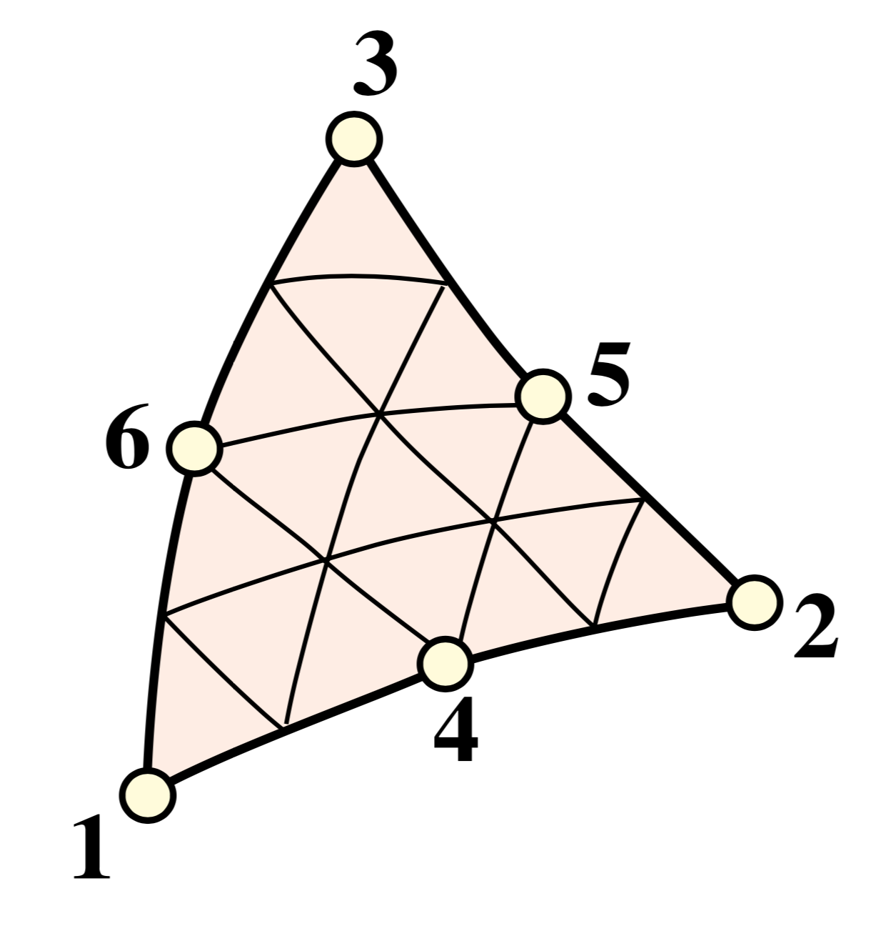
A linear (straight edged) triangle is defined by the location of it’s three vertices. However with six points, it is also possible to define what is known as a quadratic triangle, resulting in a shape with (parabolically) curved edges. These quadratic triangular elements are used in the section properties program because of their increased accuracy.

A quadratic triangular element is defined by six nodes (points), three at it's vertices and three at it's mid-sides [C. A. Felippa, Introduction to Finite Element Methods].

All you need is one element

So now we’ve managed to divide our complex shape into lots of little triangles, but none of these triangles are exactly the same. Does that mean we have to work everything out for every possible triangular shape? Luckily not! We can use isoparametric elements.

Although it has an intimidating name, the isoparametric representation has a relatively simple job. It is used to relate any conceivable triangular shape back to a basic parent shape. This way, we can do all the mathematics and programming for the simple parent shape and use isoparametric mapping to automatically relate this to more complex triangular forms! An isoparametric element has a different coordinate system to the x-y cartesian system that we’re used to. For a triangular element, this coordinate system is related to lines drawn parallel to each edge of the element.

Mapping between an isoparametric triangular element and its parent element [Samer Adeeb: http://sameradeeb.srv.ualberta.ca/].

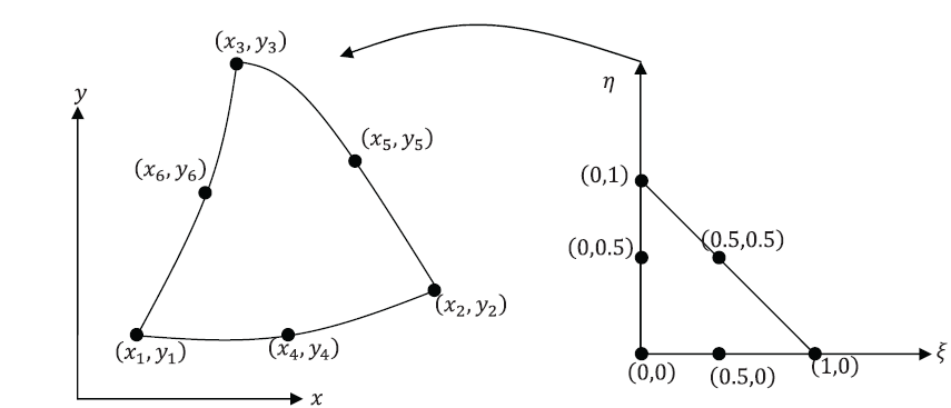
To be perfectly honest, there is some relatively complex maths behind the isoparametric mapping procedure (further details can be found here), but at the end of day, the derivation gives us three very important quantities. For a quadratic triangle, we can use it’s six definition points to compute:

• A way to interpolate a field (something that changes depending on position) within the element. This is what are known as shape functions in finite element lingo.
• A way to determine the partial derivatives of the shape functions at any point within the element.
• Something called the Jacobian, which is related to the area of the element.

With the above three quantities…

We can calculate (almost) anything!

Central to the finite element method is the integration of a changing quantity, or function, over the area of an element. In structural analysis, the assembly of the stiffness matrix involves evaluating an integral containing the partial derivatives, $\textbf{B}$:

$$\textbf{k}^e = \int_{\Omega} \textbf{B}^{\rm T} \textbf{B} \, d\Omega$$

The calculation of cross-section properties takes a similar form to this expression. The calculation of the second moment of area, for example, involves the shape functions, $\textbf{N}$, and the coordinates of the nodes, ($\textbf{y}_e$):

$$I_{xx} = \int_{\Omega} y^2 \, d\Omega = \int_{\Omega} (\textbf{N} \textbf{y}_e)^2 \, d\Omega$$

We’ve seen that with isoparametric mapping we can easily obtain the shape functions and their derivatives, but how do we evaluate the integral? The values of the above integrands are not constant within an element and are in fact polynomial functions. So does that mean we have to integrate different polynomial functions over a triangular domain?

This is where the brilliance of the German mathematician Carl Friedrich Gauss comes in. In 1814 Gauss introduced a simple formula for evaluating the integrals of polynomials by taking weighted sums at specific points, which are often referred to as Gauss points. For our quadratic triangle, if we use enough of these Gauss points, we can exactly evaluate the above integrals with just a few simple multiplications! Depending on the complexity of the integrand, we can use one of the following Gaussian quadrature rules:

One point, three point and six point Gaussian quadrature for a quadratic triangular element. Shown are the location of the Gauss points and their respective weights [C. A. Felippa, Introduction to Finite Element Methods].

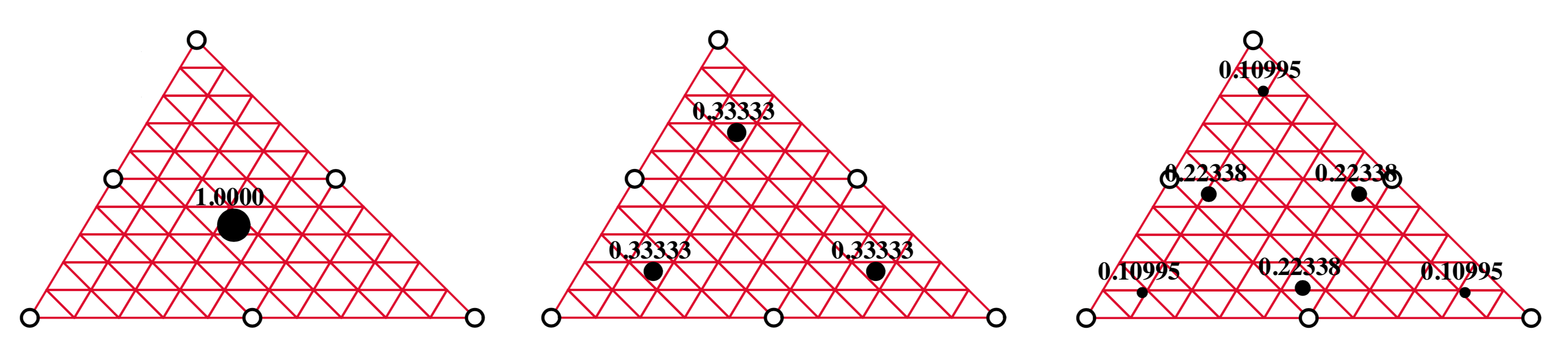
Gaussian quadrature simplifies the integral over the triangular domain to the following expression (using the second moment of area as before):

$$I_{xx} = \int_{\Omega} (\textbf{N} \textbf{y}_e)^2 \, d\Omega = \sum_{i=1}^6 w_i (\textbf{N}_i \textbf{y}_e)^2 J_e$$

where the sum is performed over six Gauss points and $J_e$ is the determinant of the Jacobian for the current Gauss point.

Bringing it all together

So now we’ve seen some of the preliminaries required to get a single finite element to work, but how do we use the theory for one small element to arrive at the section properties for a whole section?

For section properties that are not dependent on warping (more to come on this in later posts!), it’s as simple as summing the contribution of each finite element to the section property of interest. Let’s have a look at the general step-by-step process:

1. Divide the cross-section into a number of finite elements.
2. For each finite element, determine the shape functions, partial derivatives and the Jacobian.
3. For each Gauss point within the finite element, evaluate the integral relevant to the section property that is being calculated.
4. Evaluate the integral at element level by summing the weighted contribution of each Gauss point.
5. Calculate the relevant section property by summing the contribution of each finite element.

Let’s have another look at the second moment of area. Assuming we already have a finite element mesh, steps 2 to 5 might look like this in python:

# Initialise second moment of area variable
ixx = 0

# Loop through all the elements in the mesh
for el in elements:
  # Determine the Gauss points for 6pt Gaussian quadrature
  gps = gauss_points(6)

  # Loop through each Gauss point for the current element
  for gp in gps:
    # Determine the shape functions, partial derivatives and
    # Jacobian for the current Gauss point and element
    # described by coordinates xy
    (N, B, j) = shape_function(xy, gp)

    # Evaluate the integral at the current Gauss point and
    # add to the total. Note: gp[0] is the Gauss point weight,
    # xy[1,:] are the y-coordinates of the current element
    # and j is the determinant of the Jacobian
    ixx += gp[0] * (N.dot(xy[1,:])) ** 2 * j

print "ixx = {}".format(ixx)

The above procedure can be applied to most finite element analyses that involve the calculation of a quantity or the assembly of a stiffness matrix. In the upcoming blog posts I’ll be focussing more on the computation of specific section properties, which all use the above procedure in one way or another.